Task 4: Density of States calculation

Electronic density of states is an important property of a material.

$\rho(E)dE$ = number of electronic states in the energy interval $(E, E + dE)$

Calculating the Density of States (DOS) in Quantum ESPRESSO is typically a three-step process, beginning with a ground state calculation and ending with a dedicated post-processing tool.

The Three Core Steps for DOS Calculation

The standard workflow consists of the following steps:

1. Self-Consistent Field (SCF) Calculation: Run a ground state calculation using pw.x to obtain the converged charge density and wavefunctions for your system . This is the mandatory starting point for all subsequent property calculations.

2. Non-Self-Consistent Field (NSCF) Calculation: Perform a second pw.x calculation with calculation='nscf' . This step uses the charge density from the SCF run but computes the Kohn-Sham eigenvalues on a much denser k-point mesh . This dense sampling is crucial for generating a smooth and accurate DOS plot.

3. DOS Calculation with dos.x: Finally, run the dos.x executable. This program reads the data produced in the NSCF step and computes the total Density of States, outputting it to a file .

Key Input Parameters and Considerations

Here are the critical parameters for each step, along with important notes for a successful calculation.

For the NSCF (pw.x) Calculation

The input file for this step is similar to your SCF file but with key modifications:

• calculation: Must be set to 'nscf' .
• occupations: It is highly recommended to set this to 'tetrahedra' in the &SYSTEM namelist. This enables the tetrahedron method for Brillouin zone integration, which is generally more accurate for DOS than smearing techniques .
• K-Points: Define a much finer k-point grid (e.g., 12 12 12 or higher) than what was used in the SCF calculation .

For the DOS (dos.x) Calculation

This program uses a simple &DOS namelist. Below are the most important variables, based on the official documentation :

Variable	Description & Recommendations
prefix	The same prefix you used in your SCF and NSCF calculations .
outdir	The directory containing the output from your NSCF calculation .
Emin, Emax	The energy range (in eV) for the DOS plot, relative to the Fermi level .
DeltaE	The energy step (in eV) for the DOS curve. A smaller value gives a higher resolution plot .
fildos	The desired name for the output file containing the DOS data .

Important Note on the Integration Method

dos.x automatically determines the method for broadening the discrete energy levels into a continuous DOS:

• It will use the tetrahedron method if your NSCF calculation used occupations='tetrahedra' and you do not specify a degauss value in the &DOS namelist .
• Otherwise, it will fall back to Gaussian broadening, using parameters from either the &DOS namelist or the NSCF input file.

Task 4

We have created a new input file (scr/silicon/pw.scf.silicon_dos.in) which is very much the same as our previous scf input file except some parameters are modified. We used the lattice constant value that we obtained from the relaxation calculation.

We have increased the ecutwfc to have better precision. We run the scf calculation:

pw.x < pw.scf.silicon_dos.in > pw.scf.silicon_dos.out

Next, we have prepared the input file for the nscf calculation. Where is have added occupations in the &system card as tetrahedra (appropriate for DOS calculation). We have increased the number of k-points to 12 × 12 × 12 with automatic option. Also specify nosym = .TRUE. to avoid generation of additional k-points in low symmetry cases. outdir and prefix must be the same as in the scf step, some of the inputs and output are read from previous step. Here we can specify a larger number of nbnd to calculate unoccupied bands. Number of occupied bands can be found in the scf output as number of Kohn-Sham states.

pw.x < pw.nscf.silicon_dos.in > pw.nscf.silicon_dos.out

Now our final step is to calculate the density of states. The DOS input file as follows:

src/silicon/pp.dos.silicon.in

&DOS
  prefix='silicon',
  outdir='./tmp/',
  fildos='si_dos.dat',
  emin=-9.0,
  emax=16.0
/

We run:

dos.x < pp.dos.silicon.in > pp.dos.silicon.out

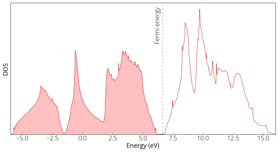
The DOS data in the si_dos.dat file that we specified in our input file. We can plot the DOS:

notebooks/silicon-dos.ipynb

import matplotlib.pyplot as plt
from matplotlib import rcParamsDefault
import numpy as np
%matplotlib inline

# load data
energy, dos, idos = np.loadtxt('../src/silicon/si_dos.dat', unpack=True)

# make plot
plt.figure(figsize = (12, 6))
plt.plot(energy, dos, linewidth=0.75, color='red')
plt.yticks([])
plt.xlabel('Energy (eV)')
plt.ylabel('DOS')
plt.axvline(x=6.642, linewidth=0.5, color='k', linestyle=(0, (8, 10)))
plt.xlim(-6, 16)
plt.ylim(0, )
plt.fill_between(energy, 0, dos, where=(energy < 6.642), facecolor='red', alpha=0.25)
plt.text(6, 1.7, 'Fermi energy', fontsize= med, rotation=90)
plt.show()

Important

For a set of calculation, we must keep the prefix same. For example, the nscf or bands calculation uses the wavefunction calculated by the scf calculation. When performing different calculations, for example you change a parameter and want to see the changes, you must use different output folder or unique prefix for different calculations so that the outputs do not get mixed.

tip

Sometimes it is important to sample the $\Gamma$ point for DOS calculation (e.g., the conducting bands cross the Fermi surface only at $\Gamma$ point). In such cases, we need to use odd k-grid (e.g., 9✕9✕5).