Task 2: Convergence tests
In practice, the user of Quantum ESPRESSO needs to make sure that simulation parameters are large enough to ensure the accuracy of the calculation. However, one cannot choose values too high or they will be spending too much computational power. Balance is key.
Automate the previous self consistent calculation by varying a certain
parameter. You can use a function that search for a keyword and updates that variable value in the input file.
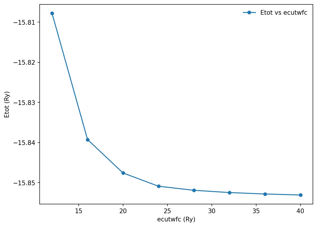
Say we want to check the total energy of the system for various
values of ecutwfc. Make a loop varying ecufwfc from 12 until 40 in steps of 4 and run the simulation for each value.
Store the total energy of calculation and plot the result.
We will use matplotlib to make the plots. Here is the python code for plotting:
import matplotlib.pyplot as plt
from matplotlib import rcParamsDefault
import numpy as np
%matplotlib inline
plt.rcParams["figure.dpi"]=150
plt.rcParams["figure.facecolor"]="white"

x, y = np.loadtxt('../src/silicon/etot-vs-ecutwfc.dat', delimiter=' ', unpack=True)
plt.plot(x, y, "o-", markersize=5, label='Etot vs ecutwfc')
plt.xlabel('ecutwfc (Ry)')
plt.ylabel('Etot (Ry)')
plt.legend(frameon=False)
plt.show()
You should get something similar to this:
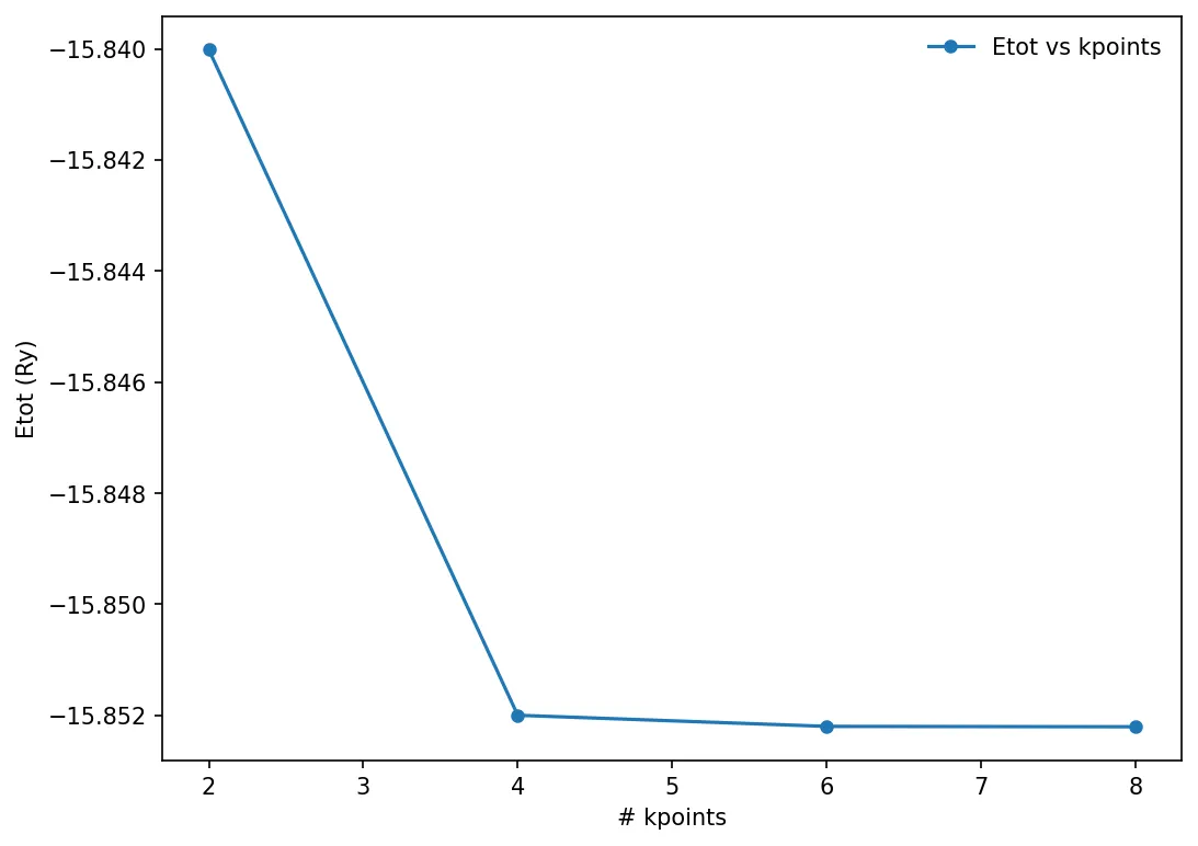
Convergence test against the number of k-points
We can run similar convergence test against another parameter, and choose the best value of that particular parameter. Here we will try to calculate the number of k-points in the Monkhorst-Pack mesh.
x, y = np.loadtxt('../src/silicon/etot-vs-kpoint.dat', delimiter=' ', unpack=True)
plt.plot(x, y, "o-", markersize=5, label='Etot vs kpoints')
plt.xlabel('# kpoints')
plt.ylabel('Etot (Ry)')
plt.legend(frameon=False)
plt.show()
Note on CPU time
-
CPU time is proportional to the number of plane waves used for the calculation. Number of plane wave is proportional to the (ecutwfc)3/2
-
CPU time is proportional to the number if inequivalent k-points
-
CPU time increases as N3, where N is the number of atoms in the system.